44.6 Sensitivity Analysis with Hazards
As described in prior sections, hazard tables can be used to represent changing health risks in many model types. To use hazard tables in a robust manner, you will also need to perform sensitivity analysis on the hazard tables to measure the impact of uncertainty.
Healthcare Example Models Hazards-PartSA-SensAn.trex illustrates one way to perform sensitivity analysis on the hazard table.
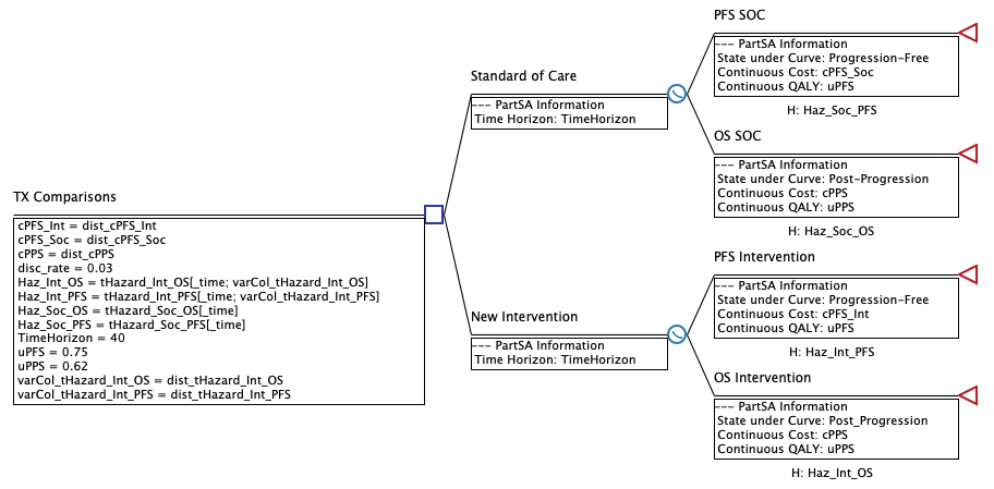
Note that the two hazard tables referenced in the New Intervention strategy include 3 columns - for low values, base case values and high values.
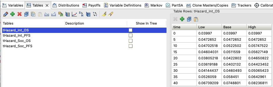
This approach provides maximum flexibility to integrate uncertainty into the hazard calculations. In the model above, you see there is no uncertainty for the first 5 years (perhaps derived from a large data set), but the uncertainty increases with time (perhaps as the data set size declines).
Before we continue with analysis of this model, let's examine Healthcare Example Models Hazards-PartSA-SensAnDisplay.trex, which specifically isolates the impact of uncertainty in the intervention strategy's OS curve.
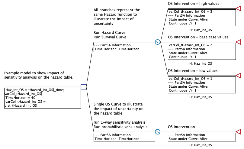
The top "strategy" of the model includes 3 branches - all of which represent the same OS curve from the prior model's Intervention strategy. The three branches represent the high, base case and low hazard values in the table by referencing a different column from the table. Select the top strategy node and run Analysis > Partitioned Survival > Hazard Curves, then Analysis > Partitioned Survival > Survival Curves.
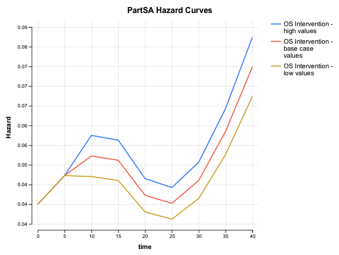
The Hazard Curves graph shows no uncertainty for the first 5 years, but then the hazard uncertainty expands to about 10% between 5 & 10 years and remains at 10% for the remainder of the time horizon as indicated by the hazard table columns.
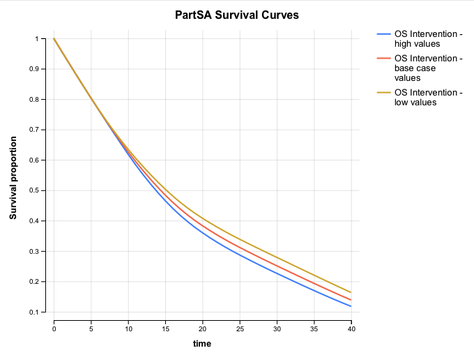
The Survival Curves graph shows the impact of that uncertainty, with no change in survival for 5 years, then and increase in uncertainty from there that drives long term differences in survival.
Now, let's examine the impact of that uncertainty on OS survival using the second strategy. That strategy contains a single OS curve, but sensitivity analyses will show the impact of the uncertainty that you will see within a model.
For deterministic sensitivity analysis, we vary the variable varCol_tHazard_Int_OS from 1-3 with 4 intervals. This will apply the values 1, 1.5, 2, 2.5 and 3 to that variable, shifting from the low hazard table column to the base case to the high hazard table column through the table lookup.
-
Haz_Int_OS = tHazard_Int_OS[_time; varCol_tHazard_Int_OS
Choose the second strategy node and run Analysis > Sensitivity Analysis > 1-way and use the default entries for variable varCol_tHazard_Int_OS.
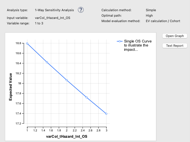
Note that as the hazard changes from the low to the high table values, the LYs accumulated drops from ~18.8 to ~17.4. In the previous model, the same impact of Intervention OS Hazard uncertainty would be applied, but it would be harder to see with the model's additional complexity.
Probabilistic sensitivity analysis (PSA) requires parameter sampling from distributions. Note that at the root node, the column variable is defined with a distribution.
-
varCol_tHazard_Int_OS = dist_tHazard_Int_OS
Let's look at how the distribution is defined in the Add/Edit Distribution dialog below.
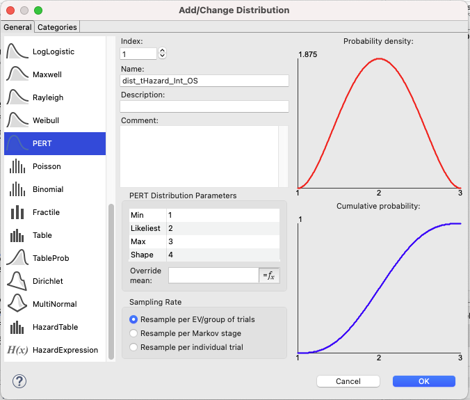
Note that the PERT distribution varies from 1 - 3, which in turn switches the hazard table column from the low values to the high values, while representing values closer to the mean of 2 more frequently than the outliers at 1 and 3.
Choose the second strategy node and run Analysis > Monte Carlo Simulation > Sampling and use the default entries in the simulation start dialog.
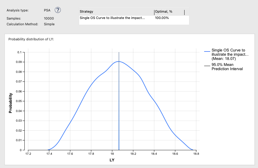
The PSA dashboard shows the same variance between LYs ~17.4 and ~18.8, but in a more realistic representation of uncertainty that does not over-represent hazard outlier values.
Now let's return to the original Healthcare Example Models Hazards-PartSA-SensAn.trex, which contains additional uncertainties beyond hazard rates.
Select the Decision Node and run Analysis > Sensitivity Analysis > Tornado Diagram, then use all the parameter uncertainties already selected. From the dashboard, choose the ICER Tornado option to see the graph below.
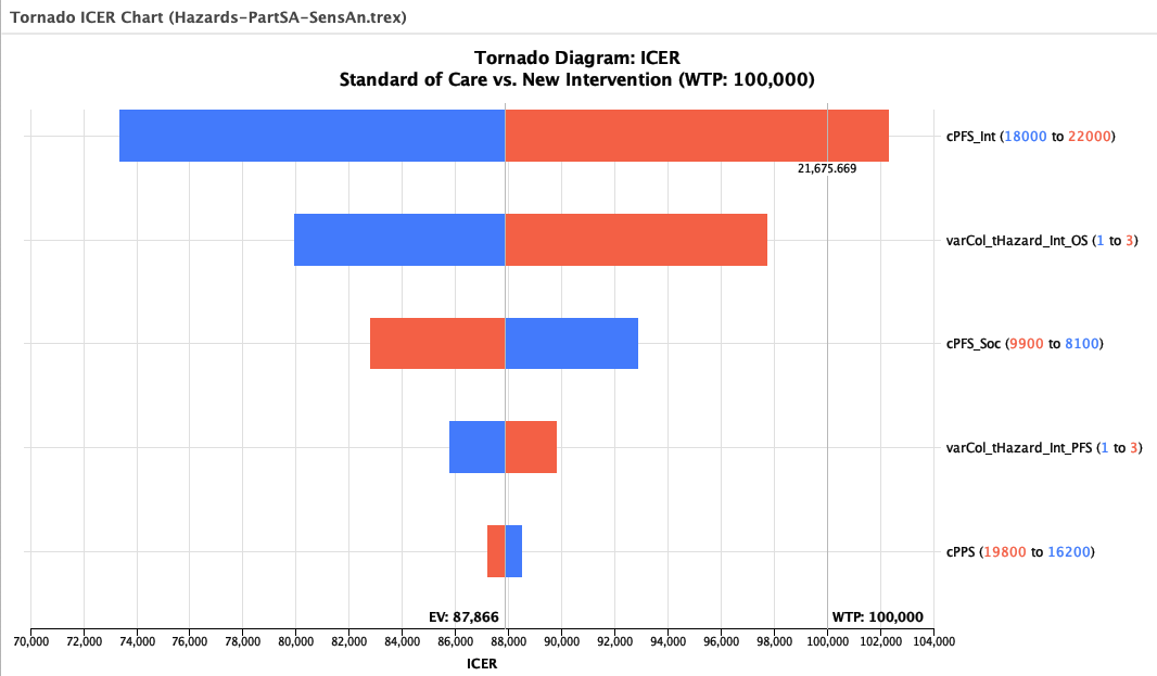
Note that the second and fourth bars represent the change in ICER caused by uncertainty in the intervention hazard values within the hazard tables.
Now return to the model and choose Analysis > Monte Carlo Simulation > Sampling to run Probabilistic Sensitivity Analysis (PSA).
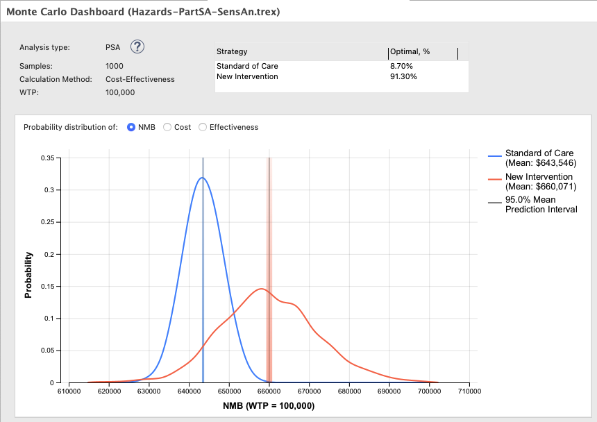
Note the range in NMB shown above is driven by a number of uncertainty distributions, including two related to hazards of the intervention strategy.
We have examined both deterministic and probabilistic sensitivity analysis on hazard tables within the context of a PartSA model, but the same techniques can be also used in Markov models, Markov Simulation models and DES models.
Also, uncertainty in hazard tables can be done with adjustment factors or formulas rather than with separate table columns. Some simple examples are includes with the Example Models. In each model, select the top "strategy" to run Hazard and Survival Curves to see the impact of sensitivity analysis by separately plotting low, base case and high hazard values, then select the bottom strategy to run sensitivity analyses.
-
Model Hazards-Sensitivity-Fixed.trex applies a fixed uncertainty factor to the hazard table entries using variable OS_Haz_SensRange and distribution dist_OS_Haz_SensRange.
-
Model Hazards-Sensitivity-Tail.trex applies a similar uncertainty factor to the hazard table entries using the same variable and distribution but gradually increasing from year 5-10 based on table applies a fixed uncertainty factor to the hazard table entriesusing variable OS_Haz_SensRange and distribution dist_OS_Haz_SensRange.
These are just a few examples. You can create any formula you wish to adjust hazards based on uncertainty.