54.8 Interpreting Calibration Results

Now, let's examine the final calibration results for our Healthcare Example Model, Calibration-Markov.trex. The results below reflect the pre-established setup, inputs and targets in the example model.

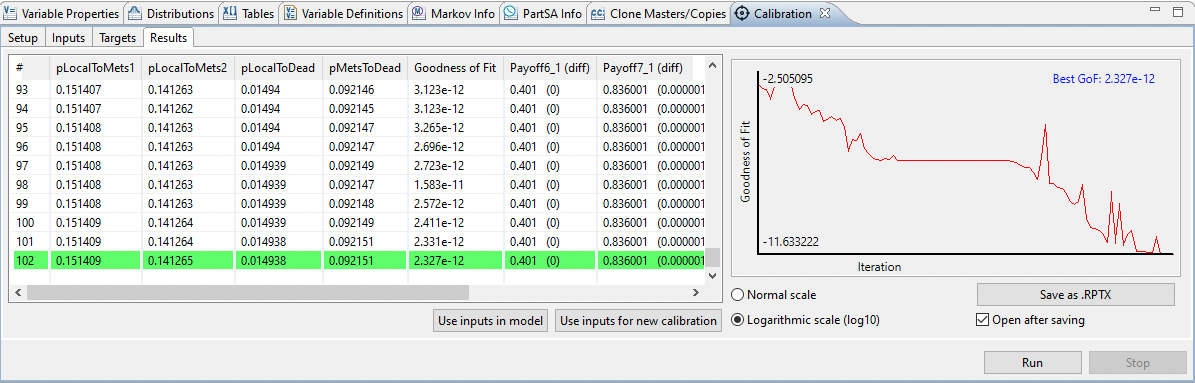
Note that the calibration process ran the model 102 times before it found a "goodness of fit" calculation within the defined tolerance.

Remember that the original model overestimated 5-year PFS and OS for both strategies, so we can expect that the calibration would increase progression probabilities to reduce survival. Let's look at the original inputs and outputs relative to those values determined by calibration. THe table below shpws the Inputs before and after calibration.

Input	Initial Value	Calibration Value
pLocalToMets1	0.15	0.151409
pLocalToMets2	0.14	0.141265
pLocalToDead	0.01	0.014938
pMetsToDead	0.10	0.092151

Note that calibration increased the probabilities for both strategies' progression and the common local cancer death probability, while the metastases death probability was slightly lower.

As a result of these changes to the inputs, we can see how the model's survival outputs now more closely match the target values. The table below shows the Outputs/targets before and after calibration

Outcome	Initial Output	Calibration Output	Target
PFS Tx 1	0.417	0.401000	0.401
OS Tx 1	0.845	0.836001	0.836
PFS Tx 2	0.442	0.426000	0.426
OS Tx 2	0.851	0.840999	0.841

Note that the calibration process was able to match up results nicely with the observed target values.

We can hope that our calibrated model is more realistic since it matches our observed data better. However, this does not guarantee that the model is perfect. You still need to start with a good model that accurately reflects disease progression.