47.2 Compound Curve Examples - Transitions
This section focuses on examples of how a modeler could use Compound Curve Transitions. The first two examples focus on survival functions rather than hazards, so they are studied solely in the PartSA context and not Markov context.
47.2.1 Transition from Table to a Fitted Distribution via Survival - Immediate
You might want to represent survival using a Kaplan-Meier table from clinical data for the observed period, then switch to a fitted parametric distribution for the extrapolation period.
The Example Model CC.1.Surv_Table_to_Dist.trex includes a Compound Curve transition which implements this.
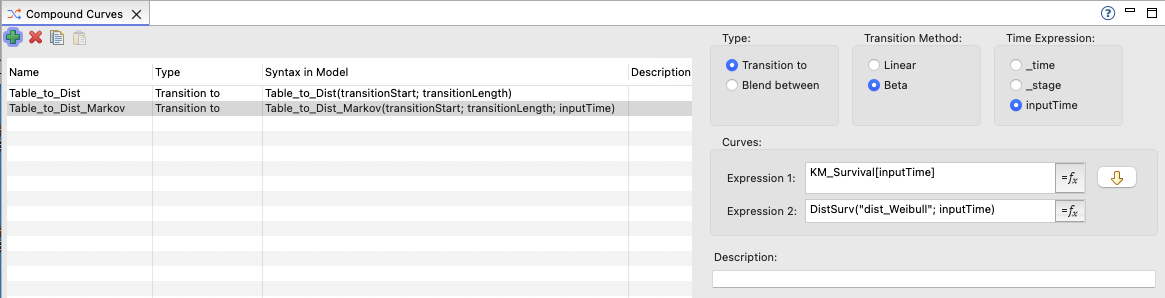
In order to create the transition, the two survival expressions must already be created in the model. The table KM_Survival contains the survival table data, and the distribution dist_Weibull represents the fitted parametric distribution from survival analysis (done external to TreeAge).
The Compound Curve transition called Table_to_Dist combines those two survival estimates as shown below. It uses the table as the initial survival expression and the distribution in the second survival expression. In Expression 2, the DistSurv function transforms the original distribution into a survival curve.
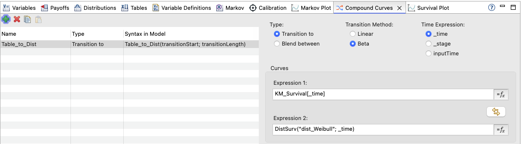
When creating the Compound Curve, the Time Expression option uses survival via _time when it is referenced in Expression 1 and 2. This would support using this Compound Curve Transition in a Partitioned Survival model but not a Markov model.
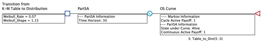
The model CC.1.Surv_Table_to_Dist.trex references the transition in the survival function for the OS curve as shown below. It uses the correct syntax as indicated in the "Syntax in Model" column when creating the compound curve (see above).
While we could run Partitioned Survival Analysis > Survival Curve for this and subsequent example models to generate and view the Survival Curve, we will instead use the Survival Plot view which can display the Survival (and Hazard) graphs. In most example models, we have setup the Survival Plot to display survival from the Compound Curve.
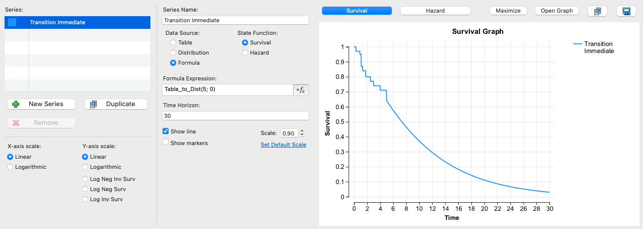
In the above Survival Plot, the Compound Curve expression Table_to_Dist(5; 0) defines survival. The syntax means it uses the Kaplan-Meier table from time 0 - 5, then at transitionStart 5 it immediately transitions (because transitionLength is 0) to the fitted distribution referenced in Expression 2. In this case, there was no need for a gradual transition because the end of the table matched to the start of the distribution at time 5.
Using the Survival Plot View means we can also review the Hazard graph as shown below (just select the button 'Hazard' above the graph).
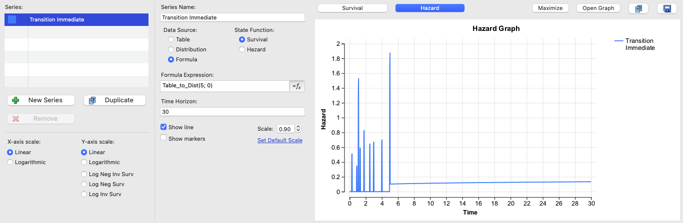
From time 0-5, the hazard is unstable due to the stepwise nature of the K-M table, then it shifts to the increasing risk associated with the Weibull distribution.
To generate Markov event probabilities from a survival-based compound curve you can use the function ProbSurvCompCurve. Example model CC.1a.Surv_Table_to_Dist.trex illustrates this technique.
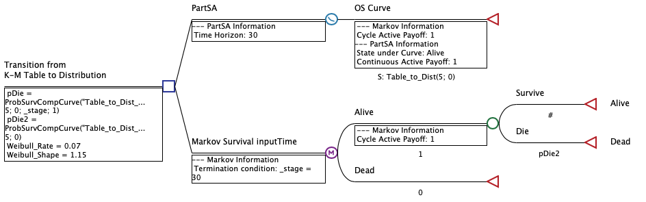
The first strategy PartSA is the same as in the previous model. The second strategy Markov Survival InputTime uses a very similar survival compound curve referencing the same table and distribution. However, the Compound Curve for the Markov model uses the time unit inputTime instead of _time to facilitate it's use with the function ProbSurvCompCurve. Note that you should always use inputTime and not _stage or _time when using the function ProbSurvCompCurve.
The two variables pDie and pDie2 perform the same calculation using different forms of the ProbSurvCompCurve function.
-
pDie = ProbSurvCompCurve("Table_to_Dist_Markov"; 5; 0; _stage; 1)
-
pDie2 = ProbSurvCompCurve("Table_to_Dist_Markov"; 5; 0)
The ProbSurvCompCurve function uses the compound curve to define survival at the beginning and the end of the cycle. It then calculates the probability required to reduce survival appropriately to match the compound curve. This function is very similar to the ProbSurvTablefunction which derives probabilities from a survival table rather than a compound curve.
Note that we strongly recommend that the underlying tables use the lookup method "interpolate" to avoid odd probability and hazard calculations from flat portions of the table.
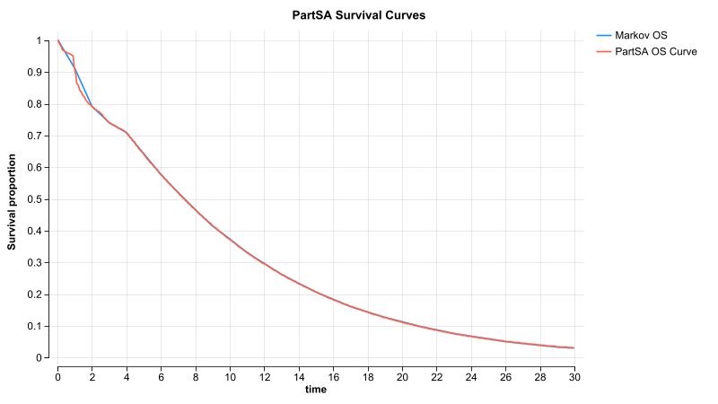
Note that the survival curves from the PartSA model and the Markov model (through cohort analysis) are nearly identical. Note that Markov survival is measured by cycle and not continuous time, so it is "smoothed out".
47.2.2 Transition from Table to a Fitted Distribution via Survival - Gradual
This is very similar to Example 1, using the same K-M table but with a different fitted distribution that does not match up closely at the transition time of 5. Since the two survival expressions do not match well, the transition from the table to the distribution is best applied gradually. The Example Model CC.2.Surv_Table_to_Dist_Gradual.trex uses the same Compound Curve transition, but in the example we show the difference with the transition applied immediately or gradually to illustrate the difference.
The Compound Curve transition Table_to_Dist combines the two survival estimates in the same way as the prior example, using the K-M table as the initial survival expression and the distribution in the second survival expression.
Again, this Compound Curve uses the Time Expression option _time, so it would support a Partitioned Survival model but not a Markov model.
Both Expressions 1 & 2 and the Time Expression reference _time, which would support using this transition in a Partitioned Survival model.
The Survival Plot view includes two series; one applying the transition immediately at transitionStart 5, the other (highlighted below) applies the transition gradually starting at transitionStart 5 and gradually applying it over transitionLength 5 (such that the expression looks like Table_To_Dist(5;5) ).
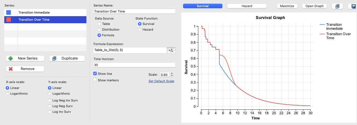
The blue curve (much of which is obstructed by the red curve) shows an immediate drop at time 5 from where the table ends and the distribution curve begins. However, the red curve gradually applies the transition, so the overall survival curve smoothly moves toward the distribution curve, resulting in a more realistic transition.
The Survival Plot's Hazard graph clearly demonstrates the difference between immediate and gradual transitionLength values.
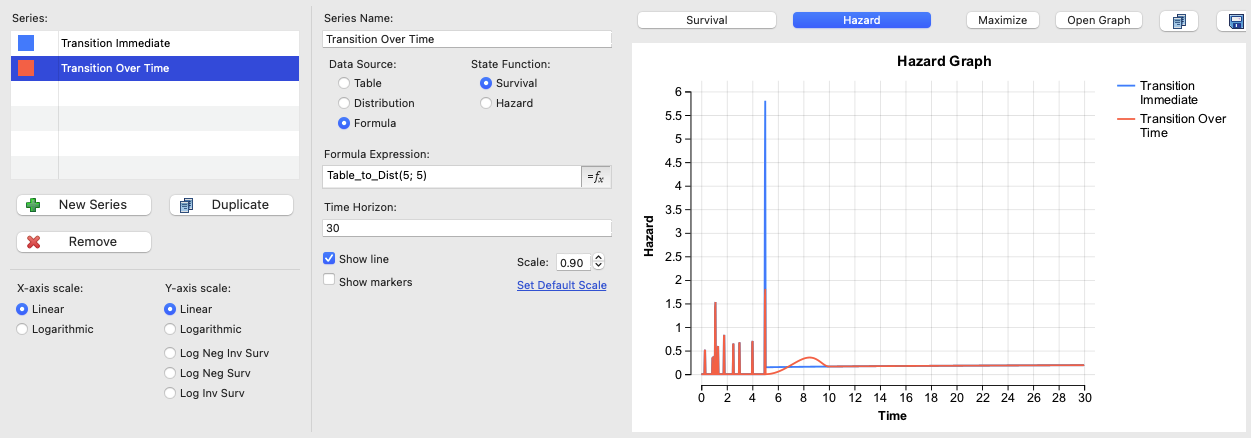
The blue curve's enormous risk/hazard applied at time 5 to force the survival curve down from the end of the table to the point on the distribution curve. The red curve applies the hazard gradually to meet the distribution curve 5 time units later.
IMPORTANT: This kind of spike or drop in hazards may indicate that using hazards to define survival may be a better approach.
47.2.3 Transition from Table to a Fitted Distribution via Hazards
This example is equivalent to the example using the Kaplan-Meier table and fitted distribution from the prior example which does not match up closely at the transition time. The Example Model CC.3.Haz_Table_to_Dist.trex uses a similar Compound Curve transition, but using hazards instead of survival. Using hazards does not require any length to the transition because the risks are applied directly to the survivors as time passes.
To use hazards in this model, the original Kaplan-Meier table had to be converted to a hazard table. During that conversion, we chose to interpolate between calculations, so the Kaplan-Meier portion of the model will be smoother than the standard Kaplan-Meier staircase. Interpolation works much better when applying hazards for Markov models, and we will look at a Markov model as well as PartSA within this example.
The PartSA Compound Curve transition Table_to_Dist_Haz begins with a hazard table in Expression 1. Expression 2 is the same distribution from the prior example, but using the DistHazard function to calculate risk over time rather than survival over time. The second Compound Curve will be discussed later in the context of a Markov model.
![]()
The first Compound Curve again uses time expression _time to support PartSA models. (The second Compound Curve that supports Markov models will be discussed later in this section.)
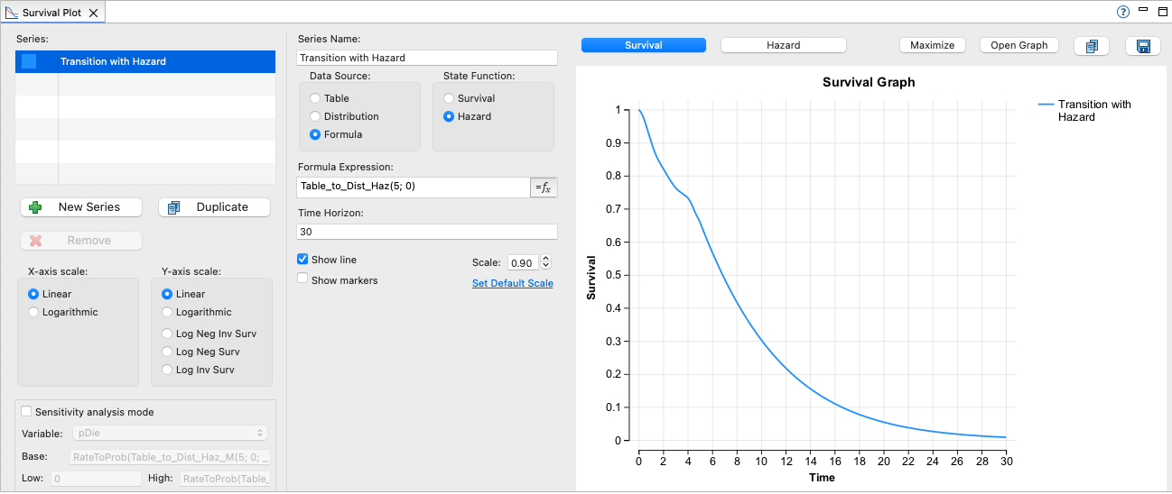
Because both the table-based and distribution-based expressions are hazards, the transition can be applied immediately because the new risk is applied directly from the point were the old risk ends, so the transition is smooth. The Survival Plot view shows the change in risk applied (immediately) at time 5.
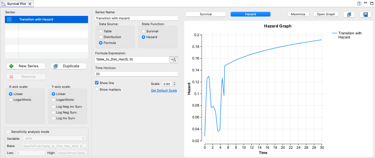
The Survival Plot's Hazard graph demonstrates the change of hazard at time 5 as well.
Markov models process based on incrementing cycles represented by _stage, so the prior Compound Curve would not work because we used Time Expression _time. For a Markov model, the Markov Compound Curve is shown below.
![]()
Note that this curve uses a time expression of inputTime rather than _time. We prefer using inputTime to _stage, so we can use the hazard halfway through the cycle to represent that time period rather than the hazard at the beginning of the cycle. However _stage would work with slightly different results.
In order to use that Markov Compound Curve, a formula is needed to convert that risk to a probability that is calculated for each cycle. This is done in a variable definition.
pDie = RateToProb( Table_to_Dist_Haz_M(5; 0; _stage+1/2); 1 )
Unwinding this variable definition, the probability is calculated by...
-
Get the hazard from the Compound Curve half way through the cycle.
-
Convert the hazard/risk to a probability for one cycle.
The variable is then referenced as the probability of death and the model runs. You can see the results in the Markov Plot.
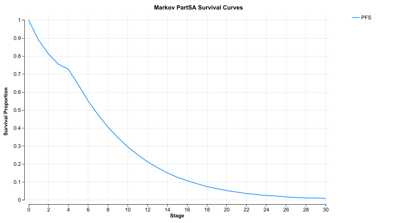
Note the Markov Plot using _stage matches nearly perfectly to the Survival Plot using _time since they are based on Compound Curves that use the same table and distribution components.
47.2.4 Transition from One Distribution to Another - Survival and Hazards
This is an example that transitions from one distribution to another distribution - but with multiple transition options. The Example Model CC.4.SurvHaz_Dist_to_Dist.trex illustrates these options using both hazards and survival (immediate vs. gradual).
There are three Compound Curve transitions.
-
Trans_Dist2_Haz transitions between two distributions using hazards via the DistHazard function.
-
Trans_Dist2_Haz_M transitions between two distributions using hazards but is used in a Markov context using the Time Expression inputTime.
-
This option could have been set to _stage, but inputTime allows us to use the hazard half-way through the cycle for that full cycle.
-
-
Trans_Dist2_Surv transitions between the distributions using survival (and hence DistSurv function).
![]()
![]()
![]()
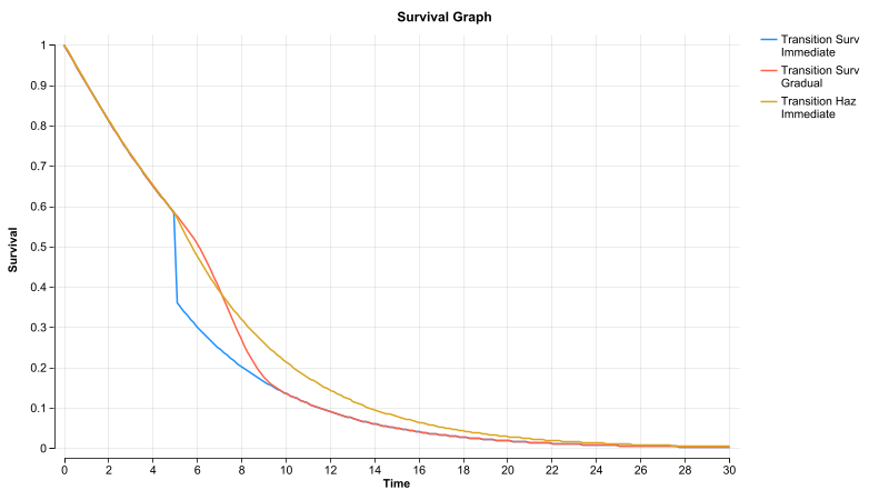
The Survival Plot view illustrates the two time-based Compound Curves in the Partitioned Survival context. Note that it can only represent the values by _time, so we can use the Markov-ready Compound Curve if we send _time in as the inputTime argument.
-
Transition Surv Immediate - transitions immediately from one survival distribution to another at time 5.
-
This forces an immediate and unnatural drop in survival at time 5.
-
-
Transition Surv Gradual - transitions gradually from one survival distribution to another at time 5 over the next 5 years.
-
This gradually adjusts survival from one distribution to the other.
-
-
Trans Haz Immediate- transitions immediately from one hazard distribution to another at time 5.
-
Note that because the new risk is applied based on where the prior left off, the transition is smooth.
-
- Trans Haz Immediate inputTime- transitions immediately from one hazard distribution to another at time 5 with the Markov-ready compound curve
We pass _time into the Survival Plot expression, but we would pass in _stage+0.5 in the Markov context.
This curve's "Show line" option is unchecked because it plots the same as the previous series.
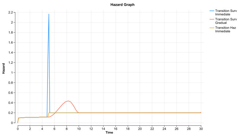
The Hazard graph from the Survival Plot illustrates the important differences between using Survival and Hazards even more clearly. There is a huge spike in hazard required to drop the survival immediately from one distribution to another. This is muted by dropping the survival gradually. When using the hazards (yellow curve) this just shifts the risk from one to another with a smooth impact on survival.
The Markov-based transition Trans_Dist2_Haz_M cannot be shown in the Survival Plot, which applies continuous _time. However, the model itself contains a Markov process that applies this transition. The results of this transition-based decline in survival can be seen in the Markov Plot.
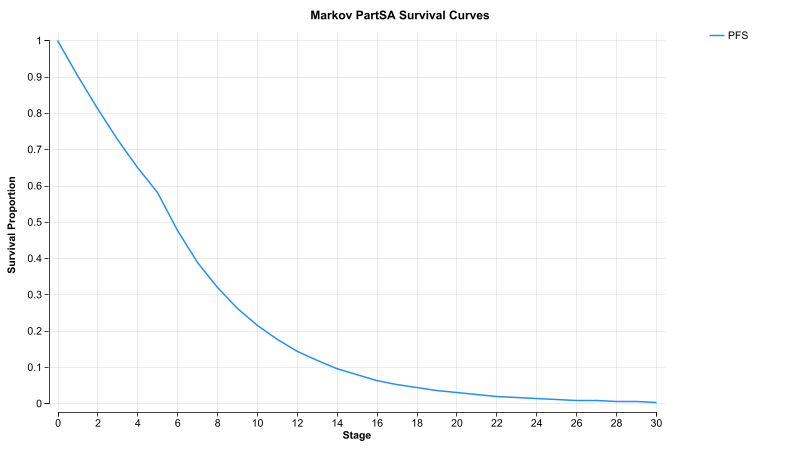
Note that the shape of the survival decline in the Markov Plot matches the hazard-based survival decline in the Survival Plot View.