13.9 Creating Correlations Among Distributions
TreeAge Pro makes it easy to create correlations among distributions for related inputs. This can be applied to parameter input distributions for Probabilistic Sensitivity Analysis on CE Models and to patient characteristics in Patient Simulation. In this section we will focus on PSA.
There are two ways to integrate correlations among distribution samples.
-
Create correlations among existing distributions to generate correlated samples.
-
Create a MultiNormal distribution that generates a set of correlated samples from normal distribution.
We recommend the first of the two approaches, so this section will focus on that with additional information at the end for the second approach.
13.9.1 Correlations Among Distributions
Model inputs can be correlated such that changes in one input are related to changes in other input(s). If you sample these inputs from independent distributions, this correlation is ignored. If correlations are ignored within the context of probabilistic sensitivity analysis, it can lead to more variance in your results than is realistic.
Input correlation can range from -1 to 1.
-
1 represents 100% correlation between inputs
-
0 represents no correlation between inputs
-
-1 represents 100% correlation in the opposite direction between inputs
Correlation among distributions is reflected in correlated samples. If there is a positive correlation, then a higher sample from the first distribution will tend to be paired with a higher sample from the second distribution. The opposite would be true if there were a negative correlation.
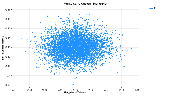
Consider the following two Custom Scatterplots showing samples from two Beta distributions with means 0.15 and 0.13, respectively. In the first graph, there is no correlation, so the samples are completely independent.
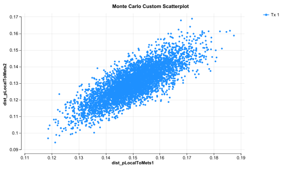
In the second graph, the distributions have a strong 0.8 correlation. Note that high samples from one are generally reflected with a high sample from the other.
To illustrated how to create such correlations, we will add correlations to Healthcare Example Model Markov-PSA-Final.trex with the correlations added in model Markov-PSA-Final-Corr.trex.
-
Open example model Markov-PSA-Final.trex.
-
Open the Distributions View.
-
Click + to add a new distribution.
-
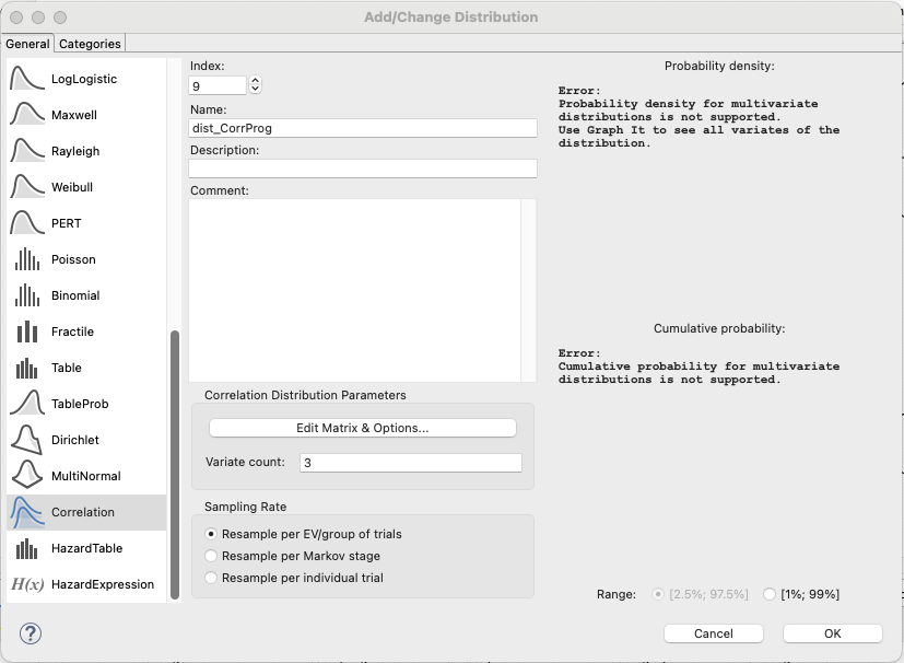
Choose the type Correlation.
-
Enter the name dist_CorrProg.
-
Click the Edit Matrix & Options button.
-
Change the Variate Count to 3 to create correlations among the 3 distributions related to progression.
-
Choose these 3 distributions along the top column header - dist_pLocalToMets1, dist_pLocalToMets2, dist_pLocalToMets3.
-
Note that you may need to expand the size of the dialog and the size of the columns.
-
-
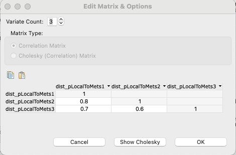
Enter correlations among the distributions as shown below then click OK.
-
Note all the correlations are positive but the strength of correlation falls from 1-2, then 1-3, then 2-3.
Click OK in the Add/Change Distribution dialog to save the new distribution.
-
Note that the new correlation dist_Corr_Prog will not be referenced directly in your model. Instead, this correlates samples from the three selected distributions dist_pLocalToMets1, dist_pLocalToMets2, dist_pLocalToMets3 which are referenced in the model.
Earlier in this section, two custom scatterplots are displayed showing the relationship among samples from the first 2 progression distributions vs. no correlation. We would see similar but slightly weaker correlations between distributions 1 and 3 and between distributions 2 and 3.
Now, let's examine the impact on overall PSA results focusing on the results from strategies 1 and 2. Because the progression probabilities are now strongly correlated, we will tend to see lower life expectancy (higher progression) or higher life expectancy (lower progression) in both strategies within the same overall model calculation.
We can see this if we look at the ICE scatterplot from the two example models. The first is from a PSA without correlation.
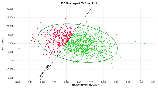
In the second graph below, there is a much smaller range of Incremental Effectiveness (IE) because there will be few pairs of sampled progression probabilities where one is very high and the other is very low. (The scale of this graph was expanded for a direct comparison to the first graph).
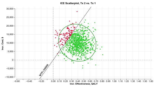
We would expect to see similar impacts of correlation in a comparison of strategies 1 & 3 and 2 & 3 since all the correlations were positive.
13.9.2 MultiNormal Distributions
Before correlations among existing distributions were added (as in the prior section), modelers used MultiNormal distributions. While this is still supported, we generally recommend the approach detailed above.
To incorporate correlations when sampling values, you can use a MultiNormal distribution. MultiNormal distributions include multiple correlated variates and generate correlated samples for each of those variates. For example, if you have three correlated inputs, you would create a single MultiNormal distribution with three correlated variates, generating three sets of correlated samples.
The rest of this section describes how to create and use MultiNormal distributions for parameters in the context of Probabilistic Sensitivity Analysis (PSA). But you could also use MultiNormal distributions for patient characteristics in the context of Patient Simulation (Microsimulation).
Correlation Example Model
The Healthcare Example Model MultiNormal Distribution Correlation.trex is a Cost-Effectiveness decision tree comparing two treatments.
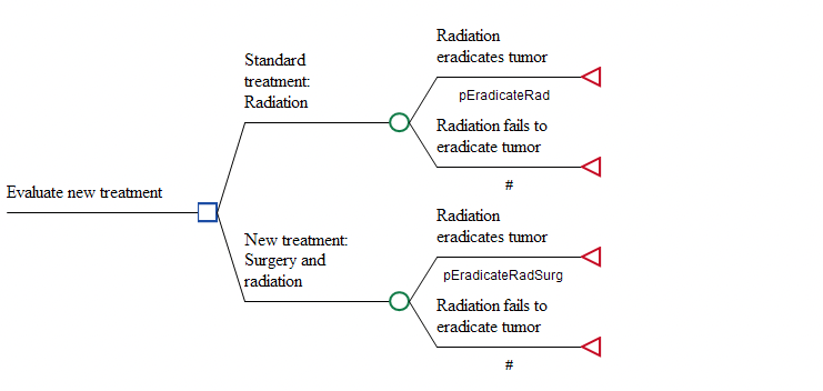
In each strategy, the patient pathways depend on the probability of eradicating the tumor. The probabilities in the two strategies are different – as represented by the variables pEradicateRad and pEradicateRadSurg.
For Probabilistic Sensitivity Analysis (PSA), those variables reference distributions. The model is set up to sample probabilities either with or without correlation between the two probability inputs. That way we can examine the impact of correlation on the PSA results.
-
No correlation – set variable correlatedSw = 0. The two probabilities are sampled from independent normal distributions.
-
Correlation – set variable correlatedSw = 1. The two probabilities are sampled from a single MultiNormal distribution which generates two correlated samples.
We will examine the results from PSA with and without correlation later in this section. Note: typically beta distributions would be used for probability parameters, but normal distributions are used in this example.
Creating a MultiNormal Distribution
Although the Example Model MultiNormal Distribution Correlation.trex used in this chapter already has the MultiNormal distribution created, this section describes how to create one.
-
Open the Distributions View.
-
Click the “+” button to create a new distribution.
-
Enter the name of the distribution.
-
Scroll down the list of distribution types to select MultiNormal.
-
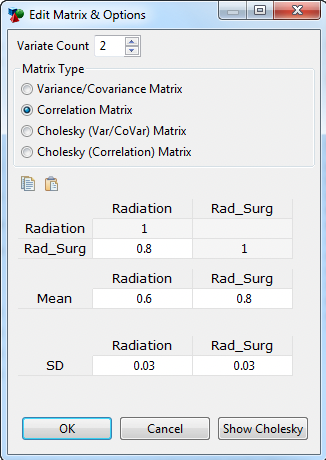
Click the Edit Matrix & Options button (See figure Screenshot #1). A second dialog “Edit Matrix & Options” will open (See figure Screenshot #2)
-
Enter the number of variates (minimum 2).
-
Select the appropriate Matrix type based on the form of your correlation data. This likely depends on the software used to generate the correlations.
-
Click on the column headings above the matrix and enter names for each variate within the MultiNormal distribution (optional) (See figure Screenshot #2 where Radiation and Rad_Surg have been entered as the column headings).
-
Enter the correlation data into the matrix grid.
-
Enter mean values for the individual variates.
-
Enter standard deviation (or scaling) values for the individual variates. Note that matrix types have variance built-in, so you would not enter the variate standard deviations.
-
If you have the matrix, mean and standard deviation data in Excel, you can copy and paste the data directly into the Matrix dialogue. Use the copy and paste buttons above the matrix.
-
Click OK to return to the Add/Change Distribution dialog.
-
In this example, the resampling rate is “Resample per EV” for use in PSA, which is what we want in this context.
-
Click OK to save the distribution.
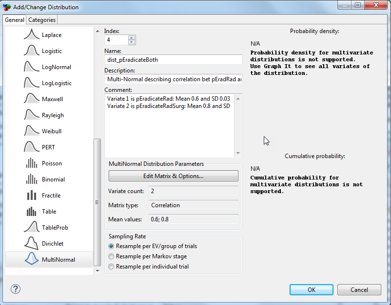
Screen shot #1
Screenshot #2
For the top two matrix types shown in Screenshot #2 above – Variance/Covariance and Correlation – TreeAge performs the Cholesky decomposition prior to sampling. Use the "Show Cholesky" button to show the calculated Cholesky Matrix as per TreeAge.
For the second two matrix types – Cholesky (Var/Covar) and Cholesky (Correlation) – the Cholesky decomposition has already been incorporated into the matrix, so TreeAge Pro does not apply it again. Depending on the software you have used to generate the correlations, you can enter data in any of these 4 formats.
Once your MultiNormal distribution is created, select the distribution in the Distributions View and click the "Graph It" icon within the Distributions View toolbar to see the samples generated for each variate of the MultiNormal distribution.
Referencing the MultiNormal Distribution in the Model
Although the Healthcare Example Model MultiNormal Distribution Correlation.trex used in this chapter already has the MultiNormal distribution incorporated, this section describes how it is referenced.
As with any distribution, it must be referenced within the model to have any impact on results. Many distributions just return a single value each time they are sampled, and these would be referenced directly, that is pVariable = dist_for_pVariable. Distributions such as MultiNormal and Dirichlet that have variates (that is they can return several values) must be referenced differently, so you can specify the variate you want. The two forms are presented below.
-
By name: Dist(“DistName”; "VariateName")
-
By index: Dist(DistIndex; VariateIndex)
You can also reference the distribution by name, and the variate by index or vice versa. Note that name entries are always placed in quotes, while index entries are not.
In our example model, the MultiNormal distribution is referenced with the first form above, but it is used only when correlationSw = 1. Therefore we see the following definitions:
-
pEradicateRad = if( correlatedSw=1 ; Dist("dist_pEradicateBoth"; "Radiation"); dist_pEradicateRad)
-
pEradicateRadSurg = if( correlatedSw=1 ; Dist("dist_pEradicateBoth"; "Rad_Surg"); dist_pEradicateRadSurg)
When running PSA with the variable correlationSw = 0, samples for the probabilities are assigned from two independent Normal distributions – dist_pEradicateRad and dist_pEradicateRadSurg. When running PSA with correlationSw = 1, samples for the probabilities are assigned from two variates of the MultiNormal distribution.
Impact of Correlation on PSA Results
To see the impact of parameter correlation, we can run PSA on the model first without correlation (correlationSw = 0), then with correlation (correlationSw = 1). In this model there is a high correlation between the parameters (0.8), so we expect the probabilities to change in a similar manner from sample to sample.
We specifically look at the ICE Scatter plot to illustrate the impact of parameter uncertainty – first without correlation, then with correlation.
PSA results - ICE Scatterplot with no correlation (correlationSw = 0)
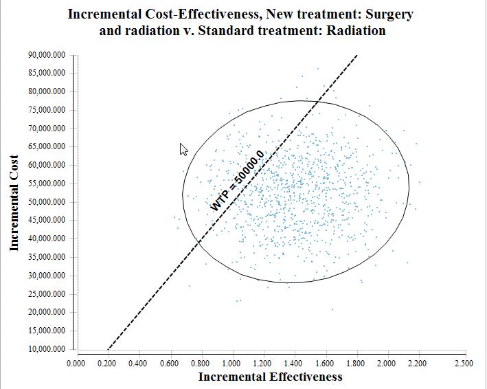
Without correlation, incremental effectiveness variance ranges from around 0.6 to 2.3.
PSA results - ICE Scatterplot with correlation (correlationSw = 1)
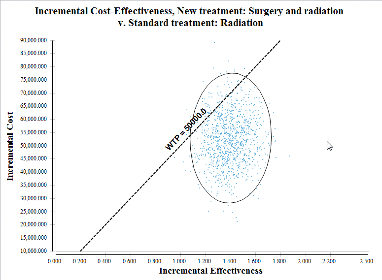
In the figures above, with correlation, incremental effectiveness variance ranges from around 0.9 to 1.8.
With high correlation between the sampled probabilities, the effectiveness values for the two strategies change together. This reduces the incremental effectiveness between the strategies' results. The reduction in the incremental cost range is less visible because incremental cost is also affected by a separate distribution dist_cSurgery.