Run Calibration and Use Adjusted Model Inputs

46.6 Run Calibration and Use Adjusted Model Inputs

Once the Setup, Inputs and Targets are ready, click the "Run" button at the bottom of the Calibration View. The Results Tab will then be selected automatically. We will run calibration on our example model MarkovCalibration_1a_Fixed_PreCal.trex.

Calibration runs in an iterative process to generate results that better match your targets in the following way:

Run the model with the initial values and compare the model outputs to the targets.
Adjust the model inputs according to the calibration algorithm.
Run the model again with the new adjusted input values and compare the model outputs to the targets.
Repeat these adjustments iteratively until the targets match within the tolerance or you reach the maximum number of model calculations.

Below are results from the Table Based Cohort calibration on the model MarkovCalibration_1a_Fixed_PreCal.trex.

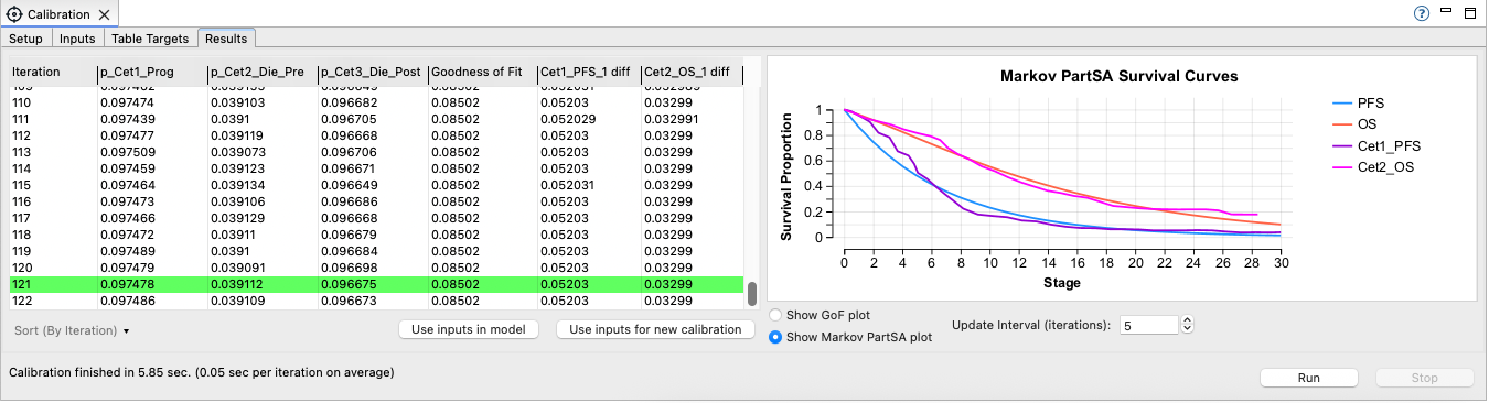
The set of inputs that find the best fit to your targets will be highlighted in green. The figure above shows the calibration stopped after 122 calculations with the 121st calculation generating the best match to targets.

Note that the results are shown as a Markov Plot by default because the calibration is matching to a single set of survival tables. This allows you to see progress in the Survival Proportion as calibration runs and the results match closer and closer to the target tables.

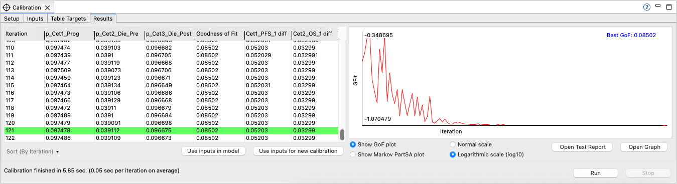
If the calibration results cannot be represented with a single set of survival tables, then the results will be displayed with the goodness of fit option as shown below.

You can stop the calibration at any time via the Stop button at the bottom right.

The Results view during/after a calibration run includes:

Results List: A list of all model calculations performed during the calculations. The results include...
- Each input value used for that calculation.
- The goodness of fit match between the model results and the targets. Note that the goodness of fit generally declines as the model results better match the targets.
- The difference between the model results and its target.
  - In a table-based calibration, this generally measures the area between the model survival curve and the clinical survival table.
- The line highlighted in green indicates the best fit identified between model outputs and targets.
Results Graph: Shows the change in the goodness of fit for each model calculation (iteration) with the "Show GoF plot" selected. You should see overall improvement in the fit overall as the process continues. We recommend viewing this with the Logarithmic scale (default), which makes it easier to see changes in the fit function over time.
Open Text Report: Open a report with all results data.
Open Graph: Open a graph showing how the results improve.

After the calibration has finished or been stopped, you can choose from these options:

Use inputs in model: Replace all the selected input values within the model with new input values from the calibration process.
Use inputs for new calibration: Replace all initial values for your calibration with new input values from the calibration process. Then you can run another calibration using the new starting point and perhaps a different algorithm.
Sort: There are options to sort the model outputs:
- By Iteration
- By Goodness of Fit (GoF) Ascending
- By GoF Descending

Note that results for the payoff-based analysis types Cohort and Microsimulation are slightly different. They are discussed later in this section.

46.6.1 Using the Calibrated Inputs in the Model

You can then use the calibrated inputs in the model by clicking the Use inputs in model button on the Run tab. This will update the root node variable definitions in the model with the best fit values from calibration.

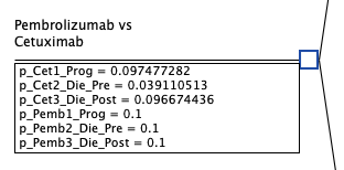
We can examine the fit between the Markov model's disease progression and the clinical tables in the Markov Plot, as seen below.

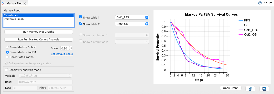
Now let's use the Markov Plot to compare the fit for the Cet strategy before calibration...

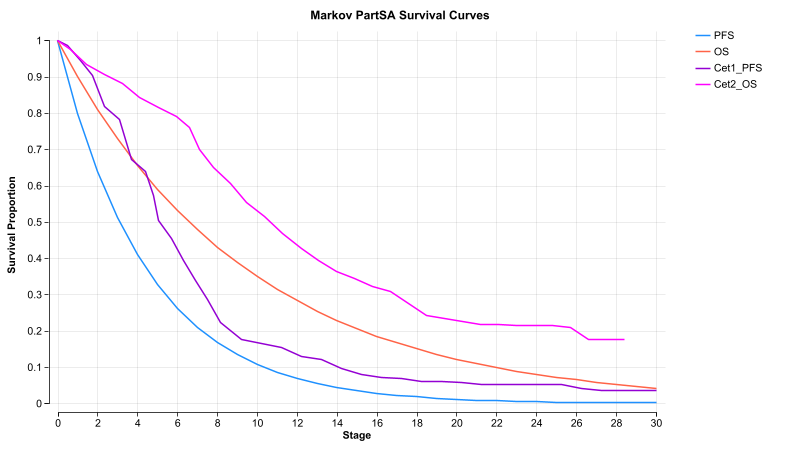
with the results and after using the calibrated inputs.

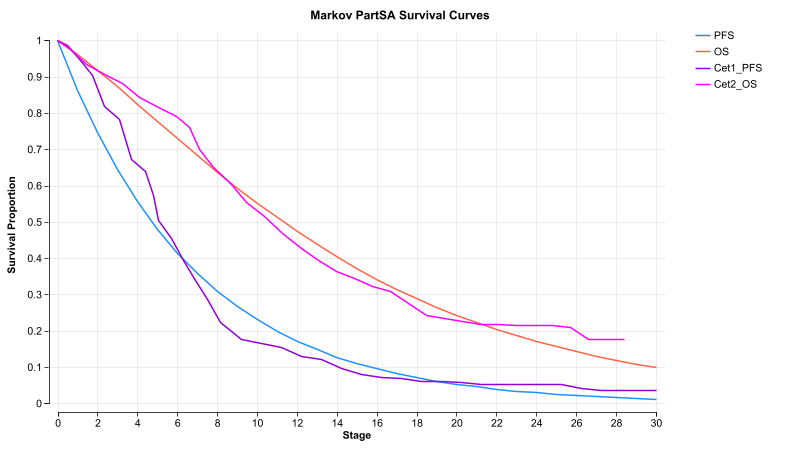
You can see visually that the calibrated results match far better to the clinical data.

Note that with fixed probabilities, we can only get so close to the clinical data. In the next section, we will run calibration on similar models where the probability allows for changing risk, as opposed to fix risk in this model. This will allow an even better fit to the clinical data.

When modeling, you can continue to edit the model structure and values, then return to calibration to match again to clinical data.

In the same model MarkovCalibration_1a_Fixed_PreCal.trex model, we can also calibrate the Pemb strategy by unchecking the Cet inputs and targets and checking the Pemb inputs and targets.

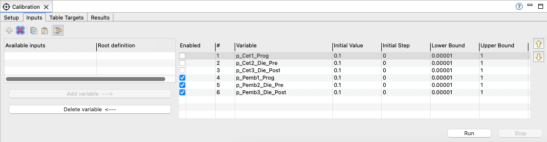
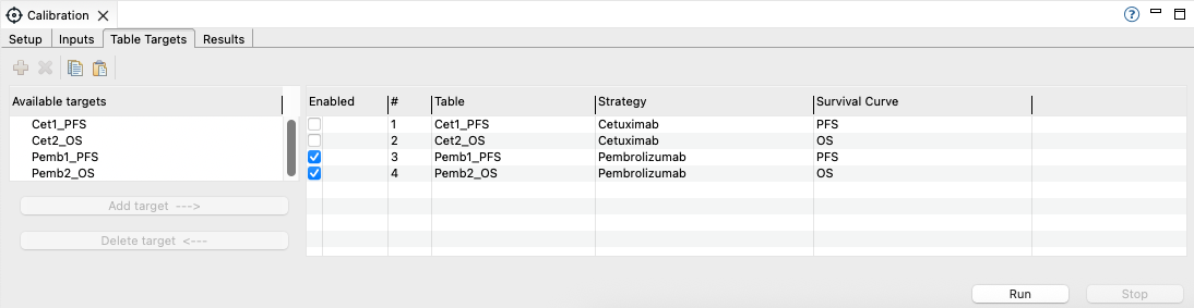
Then we can run the calibration for the Pemb strategy.

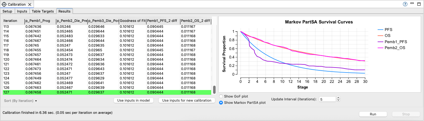
When we use those calibrated inputs in the model, the Pemb strategy results match to clinical data as well.

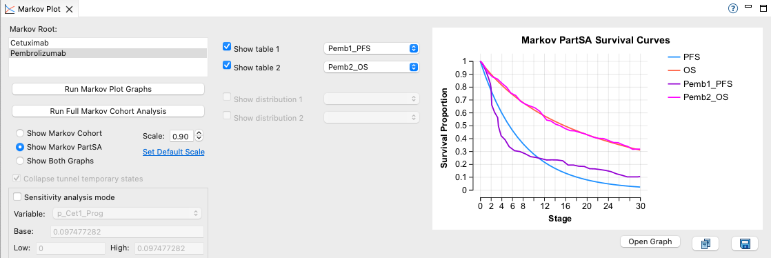
Example model MarkovCalibration_1b_Fixed_PostCal.trex includes all the calibrated inputs (as per the graphs above).

Again, we see that with fixed probabilities, we can only get so close to the clinical data. In the next section, we will run calibration on similar models where the probability allows for changing risk - providing an even better fit to the clinical data.

46.6.2 Calibration Results for Table-Based Calibration by Deterministic Range

Results will look different when you run calibration by deterministic range as the algorithm runs through every combination of input value based on the ranges and intervals. Example model MarkovCalibration_Det_PostCal.trex is setup for table-based deterministic range calibration with the Cet strategy calibration results shown below.

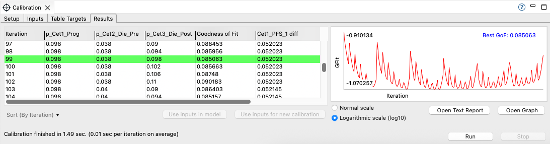
Note the pattern in the results graph as every combination of input value is run.

46.6.3 Calibration Results for Cohort and Microsimulation Analysis Types - Payoff Targets

The Cohort and Microsimulation analysis types compare model outputs (payoffs and trackers) to target values as opposed to the table-based calibration described earlier that matches model survival to clinical survival tables. Therefore the results will be presented differently.

The example model MarkovCalibration_3a_Payoffs_PreCal.trex uses payoff sets 6 and 7 to report 5-year progression-free survival and 5-year overall survival, respectively. It also uses the BOBYQA algorithm. Note the error function is based on the two selected payoffs and for each strategy. Some of the inputs affect both strategies, so a single run was used to calibrate both strategies.

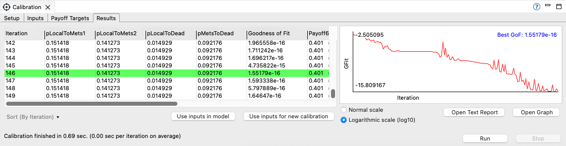
Note that the error between each payoff calculation in the model is compared to the target value for that payoff.

The Results view during/after a calibration run includes:

Results List: A list of all model results including the value for each input, the "goodness of fit" value, each calculated target ouput and the difference between the output and its target value. The best fit row is marked in green.
Results Graph: Shows the change in the goodness of fit for each model calculation (iteration). You should see overall improvement in the fit overall as the process continues. We recommend viewing this with the Logarithmic scale (default), which makes it easier to see changes in the fit function over time.
Save as *.RPTX Option: This will save the calibration output for viewing later.

After the calibration has finished or been stopped, you can choose from these functions:

Use inputs in model: This will replace all the selected input values within the model with new input values from the calibration process.
Use inputs for new calibration: This will replace all initial values for your calibration with new input values from the calibration process. Then you can run another calibration using the new starting point and perhaps a different algorithm.
Sort: There are options to sort the model outputs:
- By Iteration
- By Goodness of Fit (GoF) Ascending
- By GoF Descending

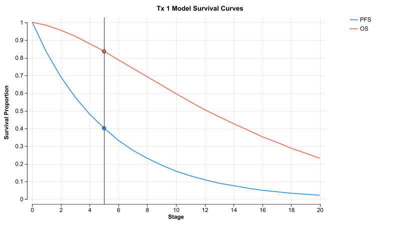
After using the calibrated inputs. Note that the 5-year PFS and Overall survival for Tx 1 matches the respective targets of 0.401 and 0.836.