46.7 Calibration with Advanced Progression Formulas

The Markov model examples we have examined so far had simple fixed probabilities for progression and death. While fixed risk may be a reasonable assumption for some models, we also know that biological risks are rarely fixed.

In this section, we will examine a few models with simple 3-state structures and more complex probability calculations.

46.7.1  Probabilities With Increasing or Decreasing Risk (Weibull)

Weibull distributions are helpful for incorporating increasing or decreasing risk into a model.

The following graphs show three distributions in the survival plot (both survival and hazard graphs). The middle series is an exponential distribution with rate 0.2. The two other series are Weibull distributions with the same rate but increasing risk (shape = 1.1) and decreasing risk (shape = 0.9).

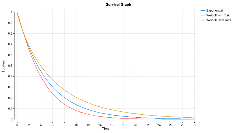
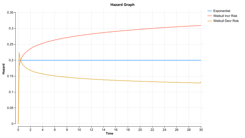
Allowing for increasing or decreasing risk allows for greater flexibility when calibrating a model.

Note that the Markov Model Wizard's calibration function auto-creates Weibull distributions to calculate event probabilities.

Consider example model MarkovCalibration_4a_Dist_PreCal.trex. Each of the six probabilities in this model is calculated from a Weibull distribution. We will examine the Cet strategy progression probability, but the rest of the probabilities are setup in the same way. The progression probability is calculated from this distribution.

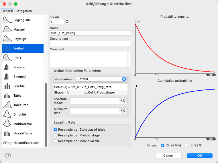
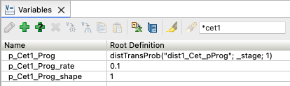
Note that the probability calculation (below) uses the DistTransProb function to reference the distribution and the parameters for the distribution are independent model inputs that can be adjusted by calibration.

With this added flexibility, we can calibrate the model strategies again, starting with the Cet strategy. Note that the rates and shapes for the three Cet probabilities are selected. Also note that the upper bound for shapes needs to be higher than 1 to allow for increasing risk.

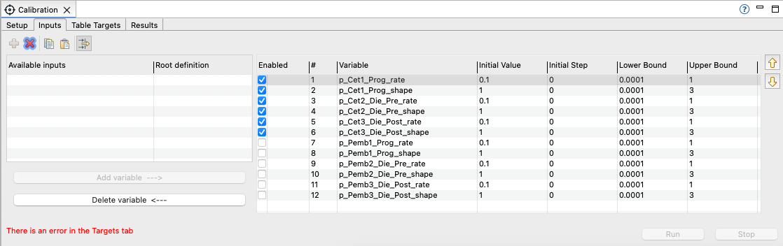
The clinical target tables are the same as earlier in this chapter - PFS and OS tables for each strategy.

Running Calibration as before, and the results are presented below. Note that some calibrated shape parameters indicate increasing risk (>1)and others decreasing risk (<1).

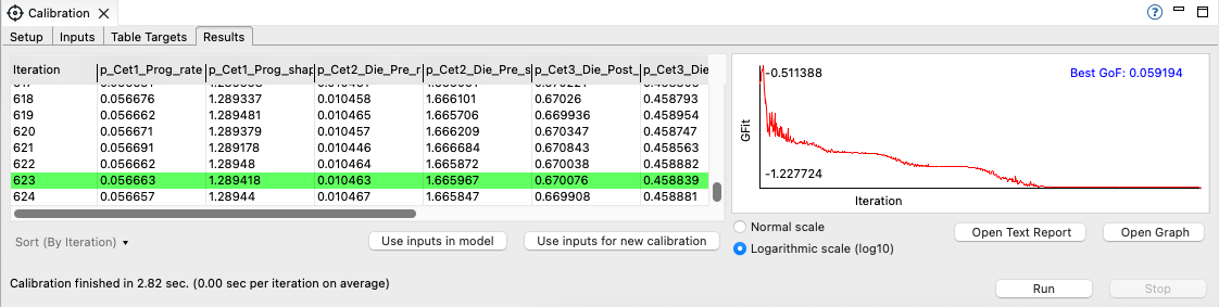
The example model with both strategies calibrated is MarkovCalibration_4b_Dist_PostCal.trex.

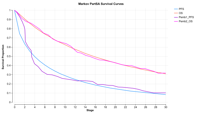
Particularly in the Pemb strategy, the calibrated inputs generate a better match with Weibull distributions as in the image below.

Compare this with the outputs which can be achieved through fixed probabilities as in the previous section (below).

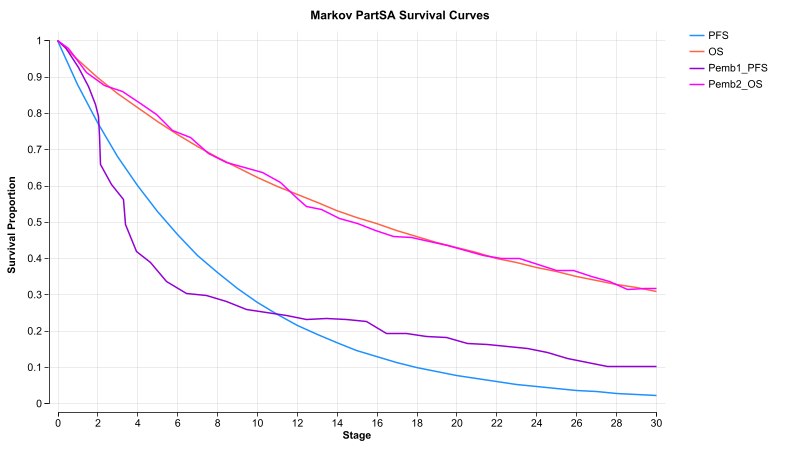
Other survival tables might find a much better fit with Weibull distributions than fixed probabilities.

46.7.2  Probabilities from Compound Curves

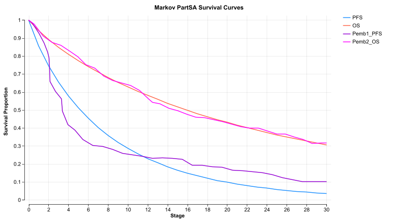
The Pemb PFS curve in our example model indicates a distinct change in risk at around time 4, suggesting a semi-curative treatment after that time. This cannot easily be modeled with a single distribution defining risk over time even using distributions.

Compound Curves provide even greater flexibility for matching clinical data by allowing for a transition from one measurement of risk to another. The example model MarkovCalibration_5a_CC_PreCal.trex includes a Compound Curve for the Pemb strategy progression probability to account for the risk change. Specifically, the Compound Curve splits the risk to use two segments based on two separate Weibull distributions.

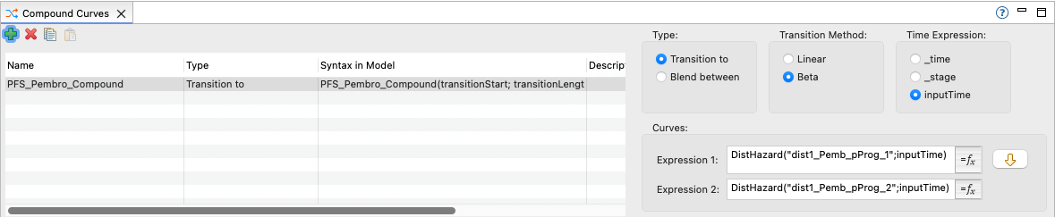
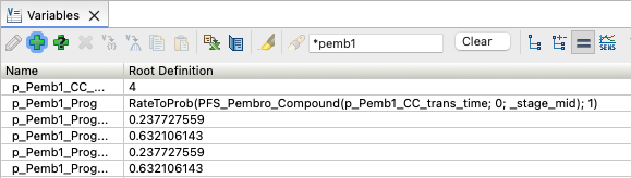
Note the variable p_Pemb1_Prog definition calculates the changing Pemb progression probability over time as follows.

• Get the risk rate at the mid-point _stage_mid from the compound curve.

  • From the first cycle through to transition time, it pulls the risk from the first distribution.

  • After the transition time, it pulls the risk from the second distribution.

• Convert the rate from the middle of the cycle to a probability to be applied over one cycle.

Prior to additional calibration, both progression distributions use the same parameters. Therefore the Compound Curve functions as if it were one distribution. We will change that with calibration. Note that the calibration inputs are setup to include the parameters for both Pemb progression distributions as well as the transition time between those distributions.

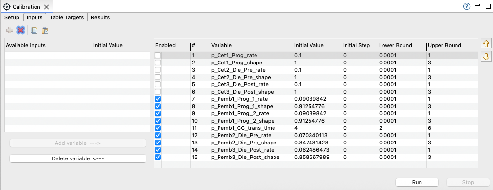
Now we can run the calibration with the same targets.

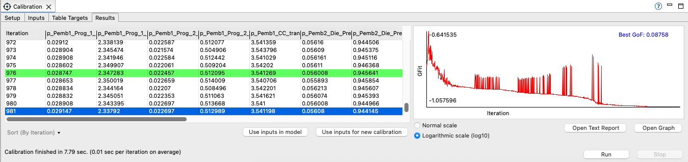
After we use the calibrated inputs in the model, we can re-examine the fit to the clinical data in the Markov Plot.

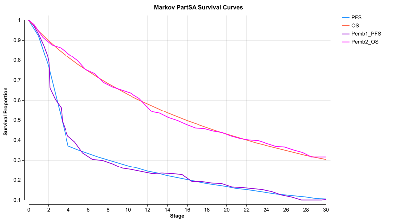
With the Compound Curve allowing the risk to shift, we now get an excellent match to the clinical survival table.

46.7.3  Adding Background Mortality

A possible issue with the prior section's model is that the curative period suggests that the risk of death declines over time even as people reach elderly ages, which is clearly not possible. Example model MarkovCalibration_BkMort_PreCal.trex includes events for background mortality calculated from CDC data.

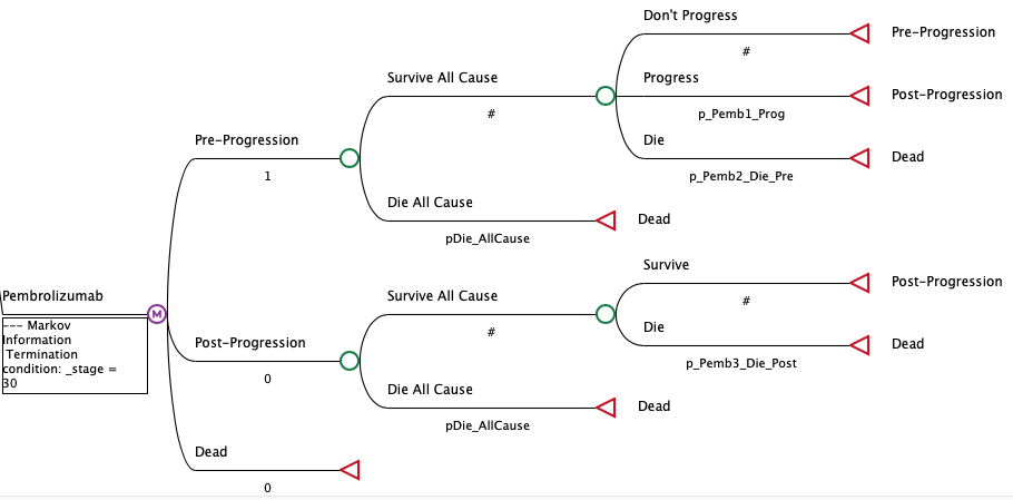
With the background mortality added, the calibrated inputs from the last section no longer generate as good a match to the clinical survival tables. In addition, we have extended the termination condition to run for 50 years starting at age 50.

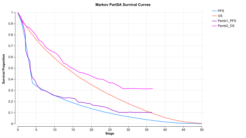
We can now run the same calibration on the Pemb strategy (same inputs and targets) on the updated model. After using the calibrated inputs, we again get a good match to the data, but not one that has unreasonable survival as the cohort nears age 100.

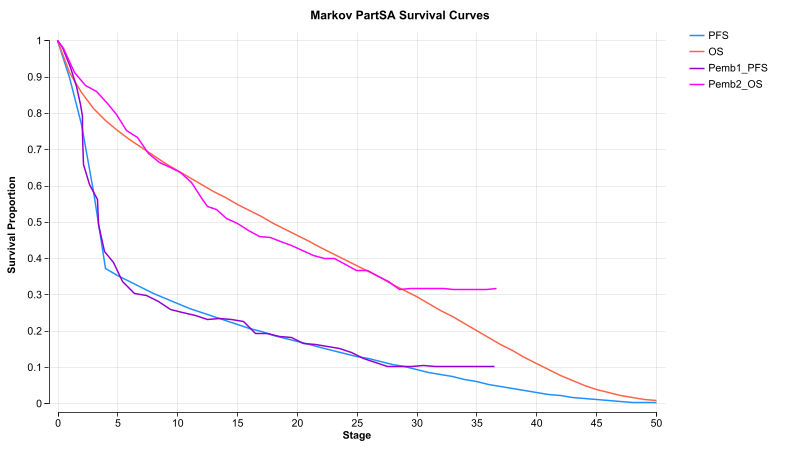
Note that after stage 30 (age 80), the model deviates from the clinical data, but this is necessary because a direct match to the data without background mortality would lead to unreasonably low death after age 80.